Empirical Bayes for Automatic Hyperparameter Tuning#
When using NormalRegressor in a contextual bandit, you must specify two hyperparameters:
``alpha`` (prior precision): Controls how strongly the model regularizes its coefficients toward zero. Too high means the model is slow to learn; too low means it overfits early data.
``beta`` (noise precision): Controls how much the model trusts individual observations. Too high means updates are too aggressive; too low means the model learns too slowly.
In practice, these are rarely known upfront. Misspecified hyperparameters lead to poor exploration-exploitation tradeoffs: the bandit either over-explores (wasting pulls on suboptimal arms) or under-explores (locking in on a suboptimal arm too early).
EmpiricalBayesNormalRegressor solves this by automatically tuning alpha and beta via evidence maximization (MacKay’s update rules). Each time the model is updated, it adjusts the hyperparameters to maximize the marginal likelihood of the observed data.
In this notebook, we demonstrate that:
A
NormalRegressorwith badly misspecified hyperparameters suffers high regretAn
EmpiricalBayesNormalRegressorinitialized with the same bad hyperparameters recovers and matches or beats a well-tuned baselineAdding a decay rate enables the EB agent to adapt to non-stationarity — when the environment shifts, the EB + decay agent tracks the new optimal hyperparameters while stationary agents stay stuck with outdated estimates
Setup: Linear Reward Oracle with Regime Shift#
We simulate a contextual bandit where the expected reward for each arm is a linear function of user features. The oracle knows the true coefficients and noise level; the bandit agents do not.
To demonstrate the value of decay, we use a two-regime data-generating process:
Phase 1 (rounds 0–2499): Large coefficients, low noise (
sigma=0.5). The optimal EB hyperparameters are low alpha (weak regularization) and high beta (trust data). Arm 0 is best on average.Phase 2 (rounds 2500–4999): Smaller coefficients, higher noise (
sigma=1.0). The optimal alpha is higher (more regularization) and optimal beta is lower. Arm 1 is now best.
This creates an environment where the stationary agents’ converged hyperparameters and learned coefficients are wrong for the second phase, while the EB + decay agent can adapt.
We use a shared model (LipschitzContextualAgent) so that all arms contribute data to a single learner. This is essential for empirical Bayes — the hyperparameter updates need sufficient data from every observation, not just the 1-in-K observations that happen to land on a particular arm.
[1]:
import numpy as np
from numpy.typing import NDArray

rng = np.random.default_rng(42)

# Phase 1: strong signal, low noise
TRUE_COEFS_1 = np.array(
    [
        [1.0, 0.5, -0.3, 0.2],  # arm 0: best on average
        [-0.5, 0.8, 0.1, -0.4],  # arm 1
        [0.3, -0.2, 0.6, 0.1],  # arm 2
        [0.0, 0.1, 0.1, 0.7],  # arm 3
    ]
)
TRUE_NOISE_STD_1 = 0.5  # beta_true = 4.0

# Phase 2: weaker signal, noisier — different optimal hyperparams
TRUE_COEFS_2 = np.array(
    [
        [0.0, 0.1, 0.1, -0.1],  # arm 0: was best, now weakest
        [0.3, 0.2, 0.3, 0.2],  # arm 1: now best (moderate, uniform)
        [-0.2, 0.1, -0.1, 0.1],  # arm 2
        [0.1, -0.1, 0.2, 0.1],  # arm 3
    ]
)
TRUE_NOISE_STD_2 = 1.0  # beta_true = 1.0

SHIFT_ROUND = 2500

N_ARMS = TRUE_COEFS_1.shape[0]
FEATURE_NAMES = ["intercept", "feature_1", "feature_2", "feature_3"]


class LinearRewardOracle:
    """Generates linear rewards with Gaussian noise."""

    def __init__(self, coefs: NDArray[np.float64], noise_std: float):
        self.coefs = coefs
        self.noise_std = noise_std
        self.context: NDArray[np.float64] = np.zeros(coefs.shape[1])

    def set_context(self, context: NDArray[np.float64]) -> None:
        self.context = context

    def expected_reward(self, arm_idx: int) -> float:
        return float(self.context @ self.coefs[arm_idx])

    def best_expected_reward(self) -> float:
        return float(np.max(self.context @ self.coefs.T))

    def generate_reward(self, arm_idx: int, rng: np.random.Generator) -> float:
        return self.expected_reward(arm_idx) + rng.normal(0, self.noise_std)


oracle = LinearRewardOracle(TRUE_COEFS_1, TRUE_NOISE_STD_1)
Defining the Arms and Agents#
We compare four agents, all using Thompson Sampling with a shared model (LipschitzContextualAgent). The arm featurizer creates block-sparse features: for arm \(a\), the user features are placed in the \(a\)-th block of a \(K \times d\)-dimensional vector (zeros elsewhere). This lets the shared model learn arm-specific coefficients — equivalent to a disjoint model, but with a single set of hyperparameters.
Default ``NormalRegressor`` (
alpha=1.0, beta=1.0) — reasonable hyperparameters that happen to work okayMisspecified ``NormalRegressor`` (
alpha=10.0, beta=0.1) — tight prior and underestimated noise precision; the model barely updates from data``EmpiricalBayesNormalRegressor`` (
alpha=10.0, beta=0.1) — same bad initialization, but EB corrects the hyperparameters automatically``EmpiricalBayesNormalRegressor`` + decay (
learning_rate=0.995) — same as above, with exponential decay to forget old data. This agent pays a regret cost in the stationary first phase, but after the regime shift it adapts while the others cannot. The estimator uses stabilized forgetting (Kulhavý & Zarrop, 1993) to continuously re-inject the EB-tuned prior, preventing it from decaying to zero.
[2]:
from bayesianbandits import (
    Arm,
    EmpiricalBayesNormalRegressor,
    FunctionArmFeaturizer,
    LipschitzContextualAgent,
    NormalRegressor,
    ThompsonSampling,
)

N_FEATURES = len(FEATURE_NAMES)


def block_sparse_featurizer(X, action_tokens):
    """Create block-sparse features: arm a gets user features in the a-th block.

    For arm a with user features x ∈ R^d, the output is:
        z_a = [0...0 | x | 0...0] ∈ R^(K*d)
    where x occupies positions [a*d : (a+1)*d].

    This lets a single shared model learn arm-specific coefficients.
    """
    n_contexts = X.shape[0]
    n_arms = len(action_tokens)
    # Output shape: (n_contexts, K*d, n_arms) — one feature vector per (context, arm) pair
    result = np.zeros((n_contexts, N_ARMS * N_FEATURES, n_arms))
    for i, token in enumerate(action_tokens):
        start = token * N_FEATURES
        end = start + N_FEATURES
        result[:, start:end, i] = X
    return result


arm_featurizer = FunctionArmFeaturizer(block_sparse_featurizer)


def make_agent(learner, seed):
    """Create a LipschitzContextualAgent with the given shared learner."""
    return LipschitzContextualAgent(
        arms=[Arm(action_token=i) for i in range(N_ARMS)],
        learner=learner,
        policy=ThompsonSampling(),
        arm_featurizer=arm_featurizer,
        random_seed=np.random.default_rng(seed),
    )


# Agent 1: Default NormalRegressor (reasonable hyperparameters)
default_agent = make_agent(NormalRegressor(alpha=1.0, beta=1.0), seed=0)

# Agent 2: Misspecified NormalRegressor (bad hyperparameters)
misspecified_agent = make_agent(NormalRegressor(alpha=10.0, beta=0.1), seed=0)

# Agent 3: Empirical Bayes (same bad initial hyperparameters, but self-correcting)
eb_agent = make_agent(EmpiricalBayesNormalRegressor(alpha=10.0, beta=0.1), seed=0)

# Agent 4: Empirical Bayes + decay (defensive against non-stationarity)
eb_decay_agent = make_agent(
    EmpiricalBayesNormalRegressor(alpha=10.0, beta=0.1, learning_rate=0.995),
    seed=0,
)
Running the Simulation#
We run all four agents for 5000 rounds on the same sequence of contexts. At round 2500, we introduce an abrupt regime shift: the true coefficients change (making a different arm optimal) and the noise level doubles. Each round, we sample a random user context, let each agent choose an arm, observe the reward, and update the agent.
[3]:
N_ROUNDS = 5000

# Pre-generate contexts so all agents see the same sequence
context_rng = np.random.default_rng(123)
contexts = np.column_stack(
    [
        np.ones(N_ROUNDS),  # intercept
        context_rng.standard_normal((N_ROUNDS, 3)),  # 3 user features
    ]
)

agents = {
    "Default (α=1, β=1)": default_agent,
    "Misspecified (α=10, β=0.1)": misspecified_agent,
    "EB (α=10, β=0.1)": eb_agent,
    "EB + decay (lr=0.995)": eb_decay_agent,
}

# Track results
optimal_rewards = np.empty(N_ROUNDS)
expected_rewards = {name: np.empty(N_ROUNDS) for name in agents}

# Track EB hyperparameters over time (both EB agents)
eb_alpha_history = []
eb_beta_history = []
eb_decay_alpha_history = []
eb_decay_beta_history = []

for t in range(N_ROUNDS):
    # Regime shift at the midpoint
    if t == SHIFT_ROUND:
        oracle.coefs = TRUE_COEFS_2
        oracle.noise_std = TRUE_NOISE_STD_2

    context = contexts[[t]]  # shape (1, 4)
    oracle.set_context(contexts[t])
    optimal_rewards[t] = oracle.best_expected_reward()

    for name, agent in agents.items():
        reward_rng = np.random.default_rng(t * 1000 + hash(name) % 1000)

        (action,) = agent.pull(context)
        arm_idx = action
        expected_rewards[name][t] = oracle.expected_reward(arm_idx)

        reward = oracle.generate_reward(arm_idx, reward_rng)
        agent.select_for_update(arm_idx).update(context, np.array([reward]))

    # Record EB hyperparameters from the shared learners
    eb_learner = eb_agent.learner
    eb_alpha_history.append(eb_learner.alpha)
    eb_beta_history.append(eb_learner.beta)

    eb_decay_learner = eb_decay_agent.learner
    eb_decay_alpha_history.append(eb_decay_learner.alpha)
    eb_decay_beta_history.append(eb_decay_learner.beta)

    if (t + 1) % 1000 == 0:
        print(f"Round {t + 1}/{N_ROUNDS}")

print("Simulation complete.")
Round 1000/5000
Round 2000/5000
Round 3000/5000
Round 4000/5000
Round 5000/5000
Simulation complete.
Results: Cumulative Regret#
Cumulative regret measures the total cost of not always choosing the best arm. Lower is better. A well-calibrated agent should achieve sublinear regret (the curve flattens over time).
[4]:
import matplotlib.pyplot as plt

fig, (ax1, ax2) = plt.subplots(1, 2, figsize=(14, 5))

colors = {
    "Default (α=1, β=1)": "C0",
    "Misspecified (α=10, β=0.1)": "C3",
    "EB (α=10, β=0.1)": "C2",
    "EB + decay (lr=0.995)": "C4",
}

for name in agents:
    regret = np.cumsum(optimal_rewards - expected_rewards[name])
    ax1.plot(regret, label=name, linewidth=2, color=colors[name])

ax1.axvline(
    x=SHIFT_ROUND, color="black", linestyle="--", alpha=0.5, label="Regime shift"
)
ax1.set_xlabel("Round")
ax1.set_ylabel("Cumulative Regret")
ax1.set_title("Cumulative Regret")
ax1.legend()
ax1.grid(True, alpha=0.3)

# Log-log scale to see sublinear behavior
rounds = np.arange(1, N_ROUNDS + 1)
for name in agents:
    regret = np.cumsum(optimal_rewards - expected_rewards[name])
    ax2.loglog(rounds, regret, label=name, linewidth=2, color=colors[name])

ax2.axvline(
    x=SHIFT_ROUND, color="black", linestyle="--", alpha=0.5, label="Regime shift"
)
ax2.set_xlabel("Round (log scale)")
ax2.set_ylabel("Cumulative Regret (log scale)")
ax2.set_title("Cumulative Regret (Log-Log)")
ax2.legend()
ax2.grid(True, alpha=0.3)

plt.tight_layout()
plt.show()

# Print final regret values
print("Final cumulative regret:")
for name in agents:
    regret = np.cumsum(optimal_rewards - expected_rewards[name])[-1]
    print(f"  {name}: {regret:.1f}")
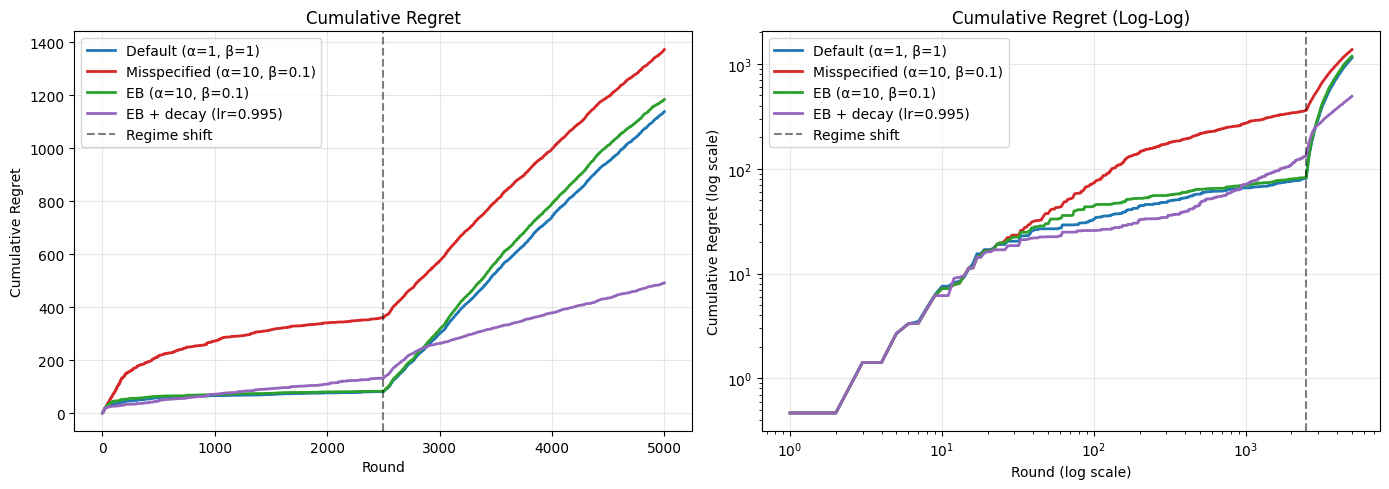
Final cumulative regret:
  Default (α=1, β=1): 1137.7
  Misspecified (α=10, β=0.1): 1371.9
  EB (α=10, β=0.1): 1183.2
  EB + decay (lr=0.995): 491.4
What to notice:
Before the regime shift (rounds 0–2499): The stationary EB agent (green) performs best — it quickly corrects its hyperparameters and exploits the strong-signal, low-noise environment. The default agent (blue) does well too. EB + decay (purple) pays a visible regret cost due to its smaller effective sample size. The misspecified agent (red) struggles throughout.
After the regime shift (rounds 2500–4999): The three stationary agents’ regret curves steepen — they’re pulling the wrong arms with outdated coefficients. The default and EB agents have accumulated so much data from phase 1 that they can’t adapt; their learned coefficients are locked in. The EB + decay agent adapts: its exponential forgetting discounts the stale phase-1 data, and the EB mechanism re-tunes the hyperparameters to the new regime. Its post-shift regret slope is noticeably lower than the others.
The key tradeoff: decay costs you regret in stationary phases but buys you adaptation when the environment changes. In this experiment, the regime shift is dramatic enough that the adaptation benefit dominates.
Hyperparameter Evolution#
The key advantage of empirical Bayes is visible in how the hyperparameters evolve. Despite starting from badly misspecified values (alpha=10, beta=0.1), both EB agents quickly adjust them toward values that better reflect the data.
In phase 1, the true noise precision is beta_true = 1 / 0.5^2 = 4.0. In phase 2, it drops to beta_true = 1 / 1.0^2 = 1.0. We expect the EB + decay agent’s beta to track this shift, while the stationary EB agent’s beta remains near its phase-1 value.
The EB + decay agent uses stabilized forgetting (Kulhavý & Zarrop, 1993): at each step, a fraction of the EB-tuned prior precision is re-injected into the model, preventing the prior from decaying to zero over time. This ensures that the EB-estimated alpha always has a channel to influence the model — and crucially, allows the hyperparameters to adapt when the optimal values change.
[5]:
fig, (ax1, ax2) = plt.subplots(1, 2, figsize=(14, 5))

# Skip the first few rounds where alpha is wildly unstable (insufficient data)
SKIP = 50

ax1.plot(
    range(SKIP, N_ROUNDS), eb_alpha_history[SKIP:], linewidth=2, color="C2", label="EB"
)
ax1.plot(
    range(SKIP, N_ROUNDS),
    eb_decay_alpha_history[SKIP:],
    linewidth=2,
    color="C4",
    linestyle="--",
    label="EB + decay",
)
ax1.axhline(y=10.0, color="C3", linestyle=":", alpha=0.7, label="Initial value (10.0)")
ax1.axvline(
    x=SHIFT_ROUND, color="black", linestyle="--", alpha=0.5, label="Regime shift"
)
ax1.set_xlabel("Round")
ax1.set_ylabel("alpha (prior precision)")
ax1.set_title("Prior Precision (alpha) Over Time")
ax1.legend()
ax1.grid(True, alpha=0.3)

ax2.plot(
    range(SKIP, N_ROUNDS), eb_beta_history[SKIP:], linewidth=2, color="C2", label="EB"
)
ax2.plot(
    range(SKIP, N_ROUNDS),
    eb_decay_beta_history[SKIP:],
    linewidth=2,
    color="C4",
    linestyle="--",
    label="EB + decay",
)
ax2.axhline(y=0.1, color="C3", linestyle=":", alpha=0.7, label="Initial value (0.1)")
# Show true noise precision for both phases
ax2.axhline(
    y=1.0 / TRUE_NOISE_STD_1**2,
    color="gray",
    linestyle=":",
    alpha=0.7,
    label=f"Phase 1 true β ({1.0 / TRUE_NOISE_STD_1**2:.1f})",
)
ax2.axhline(
    y=1.0 / TRUE_NOISE_STD_2**2,
    color="gray",
    linestyle="--",
    alpha=0.5,
    label=f"Phase 2 true β ({1.0 / TRUE_NOISE_STD_2**2:.1f})",
)
ax2.axvline(
    x=SHIFT_ROUND, color="black", linestyle="--", alpha=0.5, label="Regime shift"
)
ax2.set_xlabel("Round")
ax2.set_ylabel("beta (noise precision)")
ax2.set_title("Noise Precision (beta) Over Time")
ax2.legend()
ax2.grid(True, alpha=0.3)

plt.tight_layout()
plt.show()
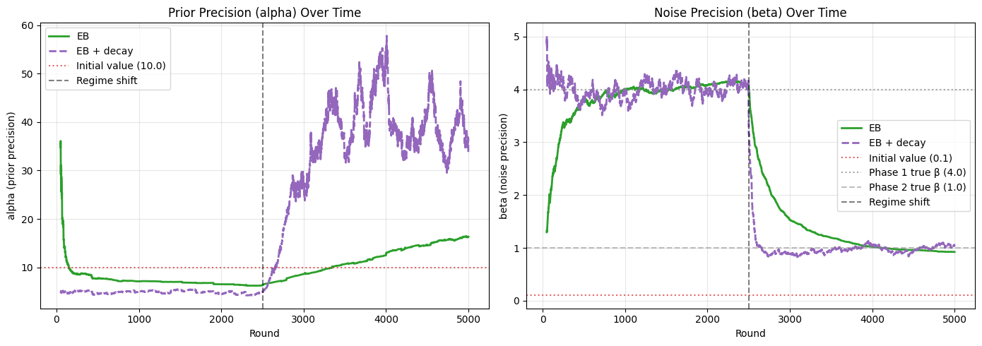
What to notice:
Phase 1 (before the dashed line): Both
alphatraces drop rapidly from 10.0 and bothbetatraces climb from 0.1 toward the true noise precision of 4.0, as in the stationary case.After the regime shift: The stationary EB agent’s (solid green) hyperparameters barely move — 2500 data points of phase-1 evidence anchor its estimates. Its
betastays near 4.0 even though the true value is now 1.0.The EB + decay agent (dashed purple) adapts: its
betadrops toward the new true value of 1.0, and itsalpharises as the weaker phase-2 signal requires more regularization. This is the mechanism behind its lower post-shift regret — the hyperparameters track the new regime because old data has been forgotten.The EB + decay traces are noisier throughout, reflecting the smaller effective sample size (~200 observations). This is the cost of adaptability.
Discussion#
When to use EmpiricalBayesNormalRegressor#
Unknown noise scale: You don’t know how noisy your rewards are (common in most real applications)
Unknown signal strength: You don’t know how large the true coefficients are, making it hard to set regularization
Sensitivity to hyperparameters: Your problem is one where bad
alpha/betavalues lead to poor performanceNo offline data for tuning: You can’t cross-validate hyperparameters before deployment
When plain NormalRegressor suffices#
Well-understood domains: You have strong prior knowledge about the noise level and coefficient scales
Offline tuning available: You can cross-validate
alphaandbetaon historical data before deploying the banditComputational budget is tight: EB adds a MacKay update step per
partial_fitcall. For most problems this overhead is negligible, but in extremely latency-sensitive applications it may matter
Decay and stabilized forgetting#
As this notebook demonstrates, decay is not just “insurance” — it is actively necessary when the environment is non-stationary. After the regime shift at round 2500:
The stationary agents (including stationary EB) accumulate regret at a steep rate because their learned coefficients and hyperparameters are locked into the phase-1 regime. With 2500 observations already incorporated, new data barely moves the posterior.
The EB + decay agent adapts: exponential forgetting discounts stale phase-1 observations, and the MacKay updates re-tune
alphaandbetato the new noise level and signal strength. The hyperparameter evolution plot shows this clearly —betadrops from ~4 toward 1 after the shift.
A naive implementation of decay causes the prior to vanish over time — after enough steps, gamma^n * alpha ≈ 0, leaving new or dormant coefficients with no regularization. EmpiricalBayesNormalRegressor addresses this with stabilized forgetting (Kulhavý & Zarrop, 1993): at each decay step, a fraction (1 - gamma) * alpha of the EB-tuned prior precision is re-injected into the precision matrix. This ensures:
The prior precision converges to
alphain steady state (instead of decaying to zero)The EB-estimated
alphaalways influences new/dormant coefficientsCold-start features receive the current population-level regularization, not a decayed remnant
The tradeoff is visible in phase 1: EB + decay pays a regret cost compared to stationary EB because its effective sample size is smaller (~200 vs 2500). In practice, the right learning_rate depends on your expected rate of environmental change — faster change warrants more aggressive decay.
Key takeaway#
The empirical Bayes approach provides robustness to hyperparameter misspecification at minimal computational cost. Pairing it with decay and stabilized forgetting adds robustness to non-stationarity — the model adapts its hyperparameters and coefficients to track a changing environment, rather than remaining anchored to stale data.